Introduction on Inference

Introduction

In this section, I learned about basic data reading in an experiment:
- Dplyr library is a powerful package used for manipulating data frames in R.
- We start by loading this package.

library(downloader)
library(dplyr)

The example for the rest of this chapter was retrived from the genomic class’s data.
Here’s how I download the dataset

url <- "https://raw.githubusercontent.com/genomicsclass/dagdata/master/inst/extdata/femaleMiceWeights.csv"
filename <- "../data/femaleMiceWeights.csv"
download(url, destfile=filename)

data <- read.csv(filename)

We can take a look at the data’s first few rows

head(data)

  Diet Bodyweight
1 chow      21.51
2 chow      28.14
3 chow      24.04
4 chow      23.45
5 chow      23.68
6 chow      19.79

For this example, I drew all the control female mice (chow) and treatment female mice (hf) into different data frames from the original dataset. Referring to the paper, the authors hypothesized that mice with treatments - a different, more fat diet would have more weights averagely than those without the treatment.
This paper was published in 2004, so the hypothesis and outcome was groundbreaking!?

control <- filter(data, Diet == "chow") %>% select(Bodyweight) %>% unlist
treatment <- filter(data, Diet == "hf") %>% select(Bodyweight) %>% unlist

print(mean(treatment))

[1] 26.83417

print(mean(control))

[1] 23.81333

obsdiff <- mean(treatment) - mean(control)
print(obsdiff)

[1] 3.020833

As we could see, the differences in the treatment was noticable when we drew from a big enough population. As I have learned, this is an indication that we can use the data earned to prove/disprove the hypothesis: “Female mice that were fed a high fat diet would earn more weights than those who weren’t”.

However, the data sampled was very random (hence the name random variables), what if I sample a different population and the results is the opposite (high fat diet makes female mice lose more weight?). The only way to make sure of this is to try and sample from a greater population, or more times, so that the results obtained are consolidated with each attempt.

I guess that is the basic of sampling and random variable to me.

Random variable

Now let’s draw from a regular, no diet population.

url <- "https://raw.githubusercontent.com/genomicsclass/dagdata/master/inst/extdata/femaleControlsPopulation.csv"
filename <- "../data/femaleControlsPopulation.csv"
download(url, destfile=filename)

population <- read.csv(filename)
population <- unlist(population)

Now we can try to sample the data many time

control <- sample(population, 12)
print(paste("Drawing once", mean(control)))

[1] "Drawing once 25.3241666666667"

control <- sample(population, 12)
print(paste("Drawing twice", mean(control)))

[1] "Drawing twice 24.8333333333333"

control <- sample(population, 12)
print(paste("Drawing for the third time", mean(control)))

[1] "Drawing for the third time 22.8433333333333"

Each sample gives a different mean of the control population. Hmmm, surely there must be a way for us to make sense of the sample average in relation to the population average?

The Null Hypothesis

Everytime we establish a hypothesis, we must concurrently establish a null hypothesis, which is the negated version of what we hypothesized. This is crucial in science, since if you want to test for something, how do you prove that it’s true? We don’t actually, the only way to test is to try and disprove it, not to prove it, as we want to make progress and advancement through “fixing” our old understanding of the subject. Science is about falsifiability, if something is omni-correct, then it’s not science, it’s not quantifiable, it’s not possible to be debunked.

sampling_times <- 10000
null <- vector("numeric", sampling_times)

for (i in 1:sampling_times) {
    control <- sample(population, 12)
    treatment <- sample(population, 12)
    null[i] <- mean(treatment) - mean(control)
}

print(mean(null >= obsdiff))

[1] 0.0143

As we can see, there’s not a lot of percentage, out of the 10000 samples, a very small percentile shows greater difference than the difference between control and treatment group above. Informally, this is known as p-value.

Probability Distributions

Distributions as my understanding, is a way to measure and make sense of the differences/variances among data within a specific metric/group. Say you have data of patients’ ages who visited the Cho Ray hospital in 2023, what can you say/describe in an overall fashion about the data? One such way is to use a CDF (cumulative distribution function).

Let’s start with a height example (because sadly I don’t have the data from Cho Ray hospital).

round(sample(x, 10), 1)

 [1] 64.7 64.6 69.3 69.3 68.6 65.1 69.2 68.6 69.6 69.6

smallest <- floor(min(x))
largest <- ceiling(max(x))
values <- seq(smallest, largest, len=300)
heightecdf <- ecdf(x)
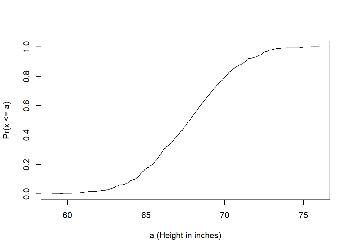
plot(values, heightecdf(values), type="l",
    xlab="a (Height in inches)", ylab="Pr(x <= a)")

The probability function explains that, “we start out with 0 example and 0 CDF, as the number of examples increase, the number of CDF also increase but you can kinda tell where most of the data lies within those examples”.

So for this data, no one was observed under ~58 inches, but there are a few at the height increases, and no further observation is greater than ~77 inches.

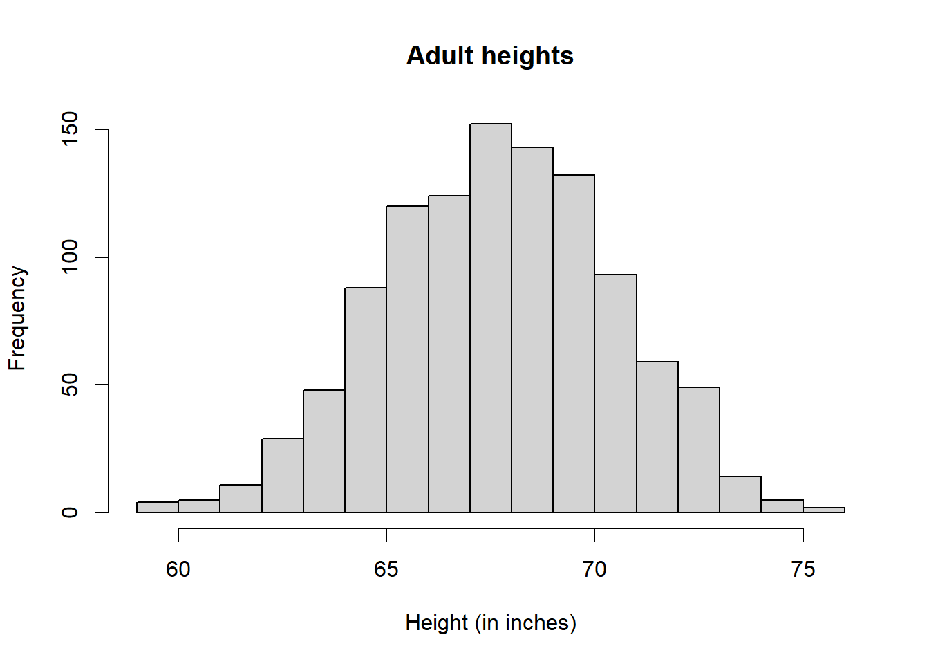
Histogram is another great way to illustrate the data:

bins <- seq(smallest, largest)
hist(x, breaks = bins, xlab = "Height (in inches)", main = "Adult heights")