Central Limit Theorem

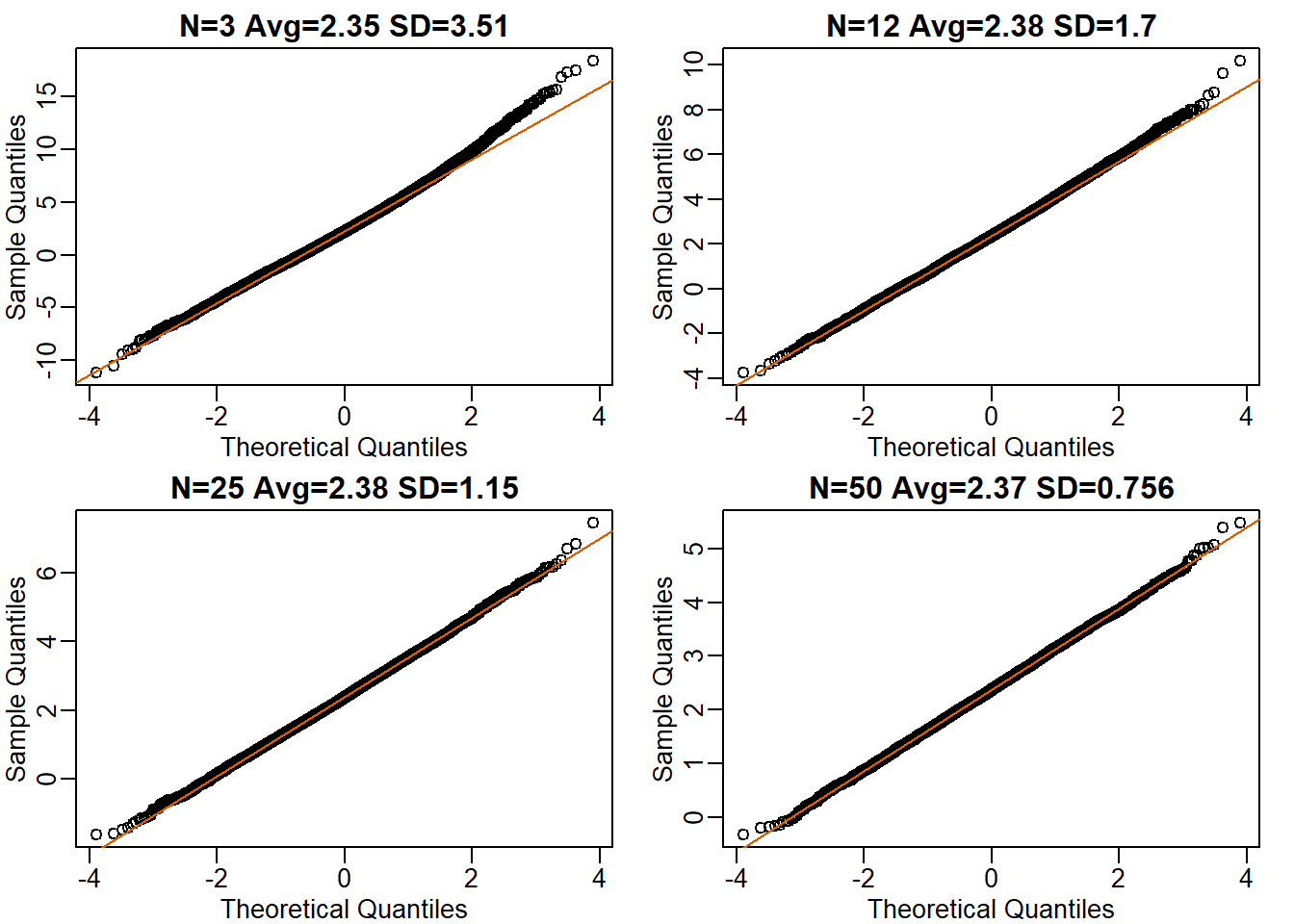
CLT is one of the most prominent theorem used in scientific computing. It tells us that once the sample size is large enough, the average of a random sample follows a normal distribution centered at the population average.

We can refer to the standard deviation of the distribution of a random variable as the random variable’s standard error.

An example for this could be the uniform change in each sample shifts the entire sample’s mean and sd by the same amount. If each mice has its own weight deducted by 10 gram, then the entire sample’s average weight would be reduced by 10 gram. Intuitively, the equation for this would be:

\[\frac{\bar{Y} - \mu}{\sigma_{Y}/\sqrt{N}}\]

t-distribution

CLT works in mostly large samples, in cases where CLT does not apply, how do we measure whether a hypothesis could be rejected or not?

T-distribution (or Student’s t-distribution) is considered when the sample size does not meet large requirements.

Let’s load an example:

library(dplyr)
library(rafalib)
library(downloader)
url <- "https://raw.githubusercontent.com/genomicsclass/dagdata/master/inst/extdata/mice_pheno.csv"
filename <- "../data/mice_pheno.csv"
download(url, destfile=filename)

dat <- read.csv("../data/mice_pheno.csv")
controlPopulation <- filter(dat, Sex == "F" & Diet == "chow") %>%  
  select(Bodyweight) %>% unlist
hfPopulation <- filter(dat,Sex == "F" & Diet == "hf") %>%  
  select(Bodyweight) %>% unlist

mypar(1,2)
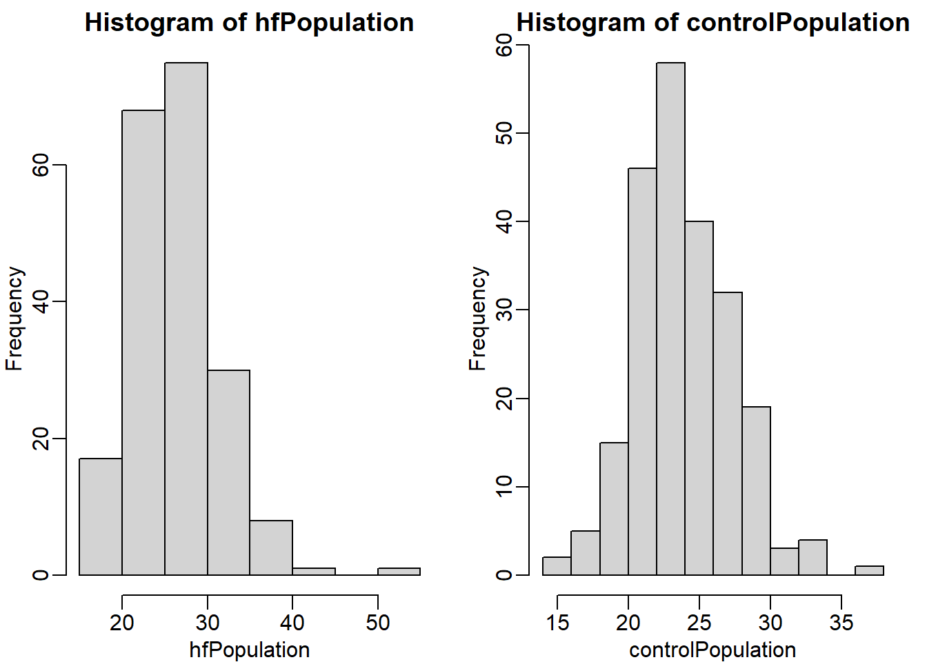
hist(hfPopulation)
hist(controlPopulation)

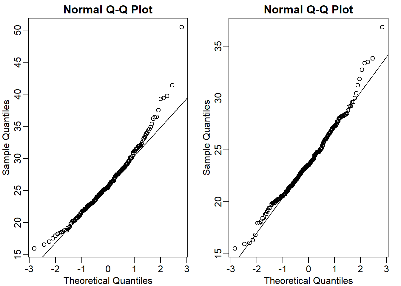
Let’s perform quartile-quartile plot to compare the distributions being closer to normal distribution.

mypar(1,2)
qqnorm(hfPopulation)
qqline(hfPopulation)
qqnorm(controlPopulation)
qqline(controlPopulation)

mu_hf <- mean(hfPopulation)
mu_control <- mean(controlPopulation)
print(mu_hf - mu_control)

[1] 2.375517

sd_hf <- popsd(hfPopulation)
sd_control <- popsd(controlPopulation)

N <- 12
hf <- sample(hfPopulation, 12)
control <- sample(controlPopulation, 12)

Ns <- c(3,12,25,50)
B <- 10000
res <-  sapply(Ns,function(n) {
  replicate(B, mean(sample(hfPopulation, n)) - mean(sample(controlPopulation, n)))
})

mypar(2,2)
for (i in seq(along=Ns)) {
  titleavg <- signif(mean(res[,i]),3)
  titlesd <- signif(popsd(res[,i]),3)
  title <- paste0("N=",Ns[i]," Avg=",titleavg," SD=",titlesd)
  qqnorm(res[,i],main=title)
  qqline(res[,i],col=2)
}